using GeoJSON, GeoExplorer, GLMakie
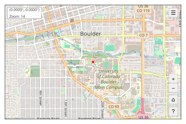
point = GeoJSON.read("""{"type": "Point", "coordinates": [-105.27, 40.01]}""")
fig = Figure(size=(600, 400))
app = explore(point; figure=fig)
wait(app.map)
save("point_example.png", fig)Getting Started
Installation
GeoExplorer.jl can be installed from the Julia package manager:
using Pkg
Pkg.add("GeoExplorer")
Basic Usage
Launching the Explorer
The simplest way to start exploring is to call explore():
using GeoExplorer

app = explore()
This opens an interactive map centered on the Continental United States using OpenStreetMap tiles.
Custom Extent
You can specify a custom initial extent:
using GeoExplorer, Extents

# View of London
app = explore(extent=Extents.Extent(X=(-0.2, 0.2), Y=(51.4, 51.6)))

# View of Tokyo
app = explore(extent=Extents.Extent(X=(139.5, 140.0), Y=(35.5, 35.9)))
Tile Providers
GeoExplorer supports multiple tile providers:
using GeoExplorer
import Tyler.TileProviders

# List available providers
providers = available_providers()

# Use Esri World Imagery (satellite)
app = explore(provider=TileProviders.Esri(:WorldImagery))

# Use CartoDB Dark Matter
app = explore(provider=TileProviders.CartoDB(:DarkMatter))

# Use Esri Topographic
app = explore(provider=TileProviders.Esri(:WorldTopoMap))
Working with Geometries
Exploring a Geometry
You can pass any GeoInterface-compatible geometry directly to explore():
using GeoExplorer, GeoJSON

# Load a GeoJSON file
geom = GeoJSON.read("my_data.geojson")

# Explore it - extent is automatically calculated
app = explore(geom)

# With custom padding around the geometry (default: 10%)
app = explore(geom, padding=0.2)  # 20% padding
Adding Geometries to an Existing Map
Use plot_geometry! to add geometries to an existing app:
using GeoExplorer, GeoJSON

app = explore()

# Load and plot a geometry
geom = GeoJSON.read("boundaries.geojson")
plot_geometry!(app, geom)

# Customize appearance
plot_geometry!(app, geom, color=:green, strokecolor=:darkgreen, strokewidth=3)
Supported Geometry Types
GeoExplorer supports all standard GeoInterface geometry types:
| Geometry Type | Default Style |
|---|---|
| Point | Red markers |
| MultiPoint | Red markers |
| LineString | Blue lines |
| MultiLineString | Blue lines |
| Polygon | Semi-transparent blue fill with blue stroke |
| MultiPolygon | Semi-transparent blue fill with blue stroke |
| GeometryCollection | Recursive plotting |
| Feature | Plots contained geometry |
| FeatureCollection | Plots all features |
multipoint = GeoJSON.read("""
{
  "type": "MultiPoint",
  "coordinates": [
    [-105.27, 40.01],
    [-104.99, 39.74],
    [-105.02, 39.65]
  ]
}
""")

fig = Figure(size=(600, 400))
app = explore(multipoint; figure=fig)
wait(app.map)
save("multipoint_example.png", fig)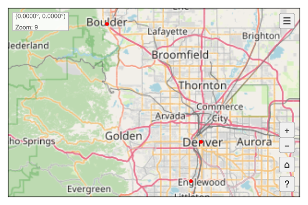
linestring = GeoJSON.read("""
{
  "type": "LineString",
  "coordinates": [
    [-105.27, 40.01],
    [-104.99, 39.74],
    [-104.82, 39.55],
    [-104.76, 39.10]
  ]
}
""")

fig = Figure(size=(600, 400))
app = explore(linestring; figure=fig)
wait(app.map)
save("linestring_example.png", fig)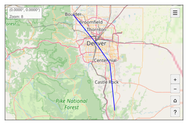
multilinestring = GeoJSON.read("""
{
  "type": "MultiLineString",
  "coordinates": [
    [[-105.5, 40.0], [-105.0, 40.0], [-104.5, 40.0]],
    [[-105.5, 39.5], [-105.0, 39.5], [-104.5, 39.5]],
    [[-105.5, 39.0], [-105.0, 39.0], [-104.5, 39.0]]
  ]
}
""")

fig = Figure(size=(600, 400))
app = explore(multilinestring; figure=fig)
wait(app.map)
save("multilinestring_example.png", fig)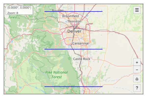
polygon = GeoJSON.read("""
{
  "type": "Polygon",
  "coordinates": [[
    [-105.3, 40.1],
    [-105.1, 40.1],
    [-105.1, 39.9],
    [-105.3, 39.9],
    [-105.3, 40.1]
  ]]
}
""")

fig = Figure(size=(600, 400))
app = explore(polygon; figure=fig)
wait(app.map)
save("polygon_example.png", fig)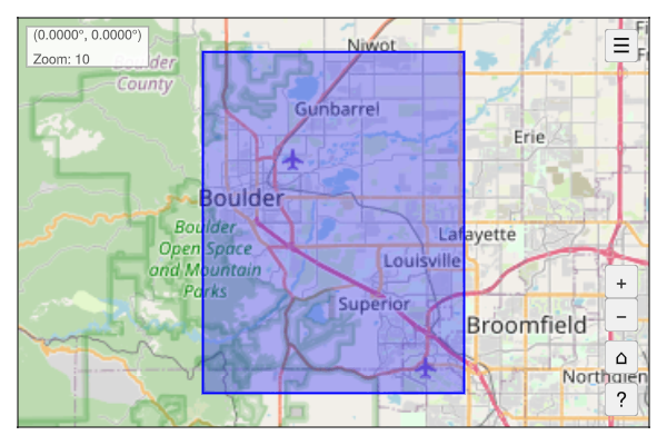
multipolygon = GeoJSON.read("""
{
  "type": "MultiPolygon",
  "coordinates": [
    [[[-105.3, 40.1], [-105.1, 40.1], [-105.1, 39.95], [-105.3, 39.95], [-105.3, 40.1]]],
    [[[-105.1, 39.85], [-104.9, 39.85], [-104.9, 39.7], [-105.1, 39.7], [-105.1, 39.85]]]
  ]
}
""")

fig = Figure(size=(600, 400))
app = explore(multipolygon; figure=fig)
wait(app.map)
save("multipolygon_example.png", fig)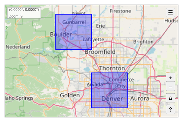
featurecollection = GeoJSON.read("""
{
  "type": "FeatureCollection",
  "features": [
    {
      "type": "Feature",
      "properties": {"name": "Boulder"},
      "geometry": {"type": "Point", "coordinates": [-105.27, 40.01]}
    },
    {
      "type": "Feature",
      "properties": {"name": "Denver"},
      "geometry": {"type": "Point", "coordinates": [-104.99, 39.74]}
    },
    {
      "type": "Feature",
      "properties": {"name": "Route"},
      "geometry": {
        "type": "LineString",
        "coordinates": [[-105.27, 40.01], [-104.99, 39.74]]
      }
    }
  ]
}
""")

fig = Figure(size=(600, 400))
app = explore(featurecollection; figure=fig)
wait(app.map)
save("featurecollection_example.png", fig)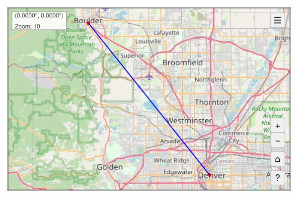
Working with Layers
Layers allow you to manage multiple data overlays with visibility controls.
Adding Layers
using GeoExplorer, GLMakie

app = explore()

# Plot data and register as a layer
xs, ys = [...], [...]  # Web Mercator coordinates
plt = scatter!(app.map_axis, xs, ys; color=:red)
add_layer!(app, "My Points", plt)

# Add another layer
line_plt = lines!(app.map_axis, xs, ys; color=:blue)
add_layer!(app, "Connections", line_plt)
Layer Controls
Click the layers button (☰) in the top-right to:
- Toggle layer visibility with checkboxes
- Zoom to a layer’s extent with the zoom button (⌖)
Programmatic Layer Control
# Toggle visibility
toggle_layer!(app, "My Points")

# Zoom to layer extent
zoom_to_layer!(app, "My Points")

# Get a layer by name
layer = get_layer(app, "My Points")

# Remove a layer
remove_layer!(app, "My Points")
Using with Geocoding
GeoExplorer works well with geocoding packages:
using GeoExplorer, OSMGeocoder

# Geocode a city and explore it
result = geocode(city="Boulder", state="CO")

app = explore(result)