MatrixFreeOperators.jl

Welcome to the documentation for MatrixFreeOperators.jl.

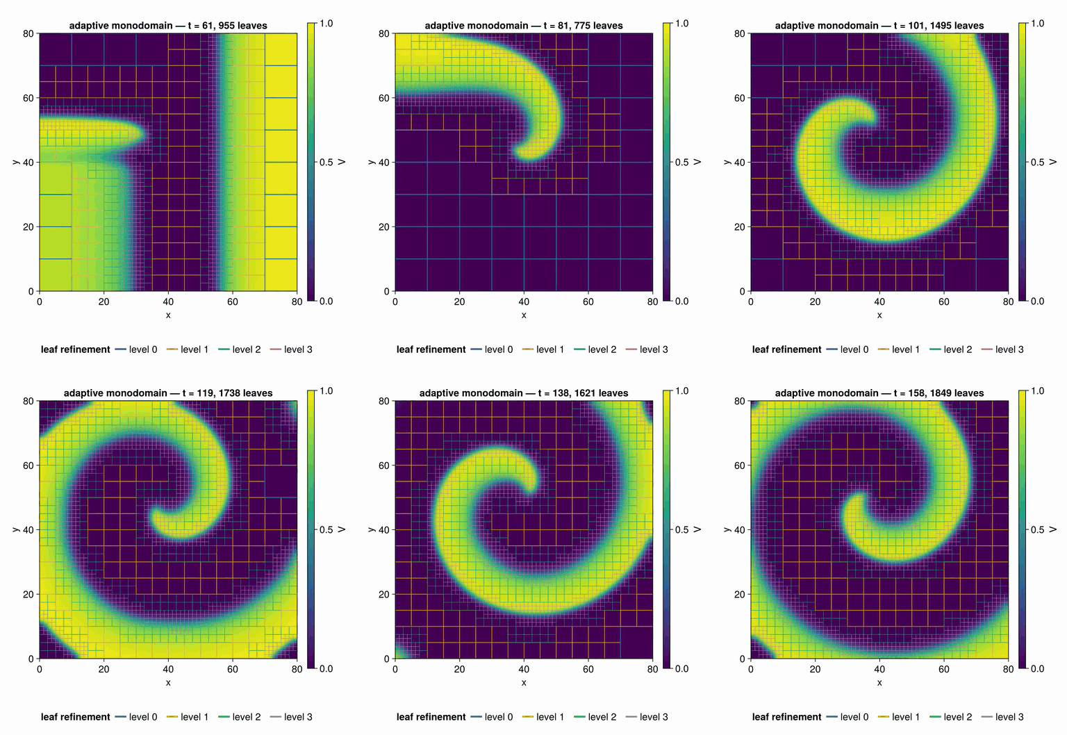
Animated cardiac electrophysiology simulation: a spiral wave rotating on an adaptively refined block mesh whose fine blocks track the wavefront. — Aliev–Panfilov monodomain cardiac electrophysiology on an adaptive `BlockForest`. `regrid!` refines on |∇V|, so resolution tracks the depolarization wavefront and coarsens behind it while an S1–S2 protocol breaks a planar wave into a reentrant spiral. Source: `examples/monodomain_amr.jl`.

Overview

MatrixFreeOperators.jl provides matrix-free linear (and some nonlinear) operators for solving PDEs on structured grids. Operators are lazy, composable symbols (laplacian, gradient, divergence, scaling, advection, …) combined with +, -, *, and scalar scaling. Leaves are written as array-level broadcasts, so the same operator runs on CPU and GPU arrays, differentiates automatically — Enzyme is the default backend, DifferentiationInterface the recommended frontend, and gradients extend to operator parameters such as material-coefficient fields (see Automatic Differentiation) — and feeds Krylov.jl directly through prepare + mul! with zero steady-state allocations. Explicit time stepping skips that flat boundary — a hand-rolled stepper calls the field-level apply!(du, L, u), as in examples/heat_equation.jl; there is no OrdinaryDiffEq.jl integration yet (#81). When one device is not enough, prepare_distributed partitions the grid across several GPUs without changing a line of operator code — see Distributed Multi-GPU Solves. If you are here to change the package rather than use it, Internals walks each main operation’s call sequence with the concrete types named at every step.

Quickstart

using MatrixFreeOperators, Krylov, LinearAlgebra

# -Δu + σu = f on (0,1)², homogeneous Dirichlet, manufactured solution
g = CartesianGrid(((0.0, 1.0), (0.0, 1.0)), (32, 32))
σ = set!(scalar_field(g), x -> 1 + x[1] * x[2])
K = scaling(σ) - laplacian(g)

f = set!(scalar_field(g), x -> (2π^2 + 1 + x[1] * x[2]) * sinpi(x[1]) * sinpi(x[2]))
P = prepare(K, scalar_field(g))
u, stats = cg(P, flatten(f))

maximum(abs, u .- flatten(set!(scalar_field(g), x -> sinpi(x[1]) * sinpi(x[2]))))

0.0007541253359059086