MatrixFreeOperators.jl

Welcome to the documentation for MatrixFreeOperators.jl.

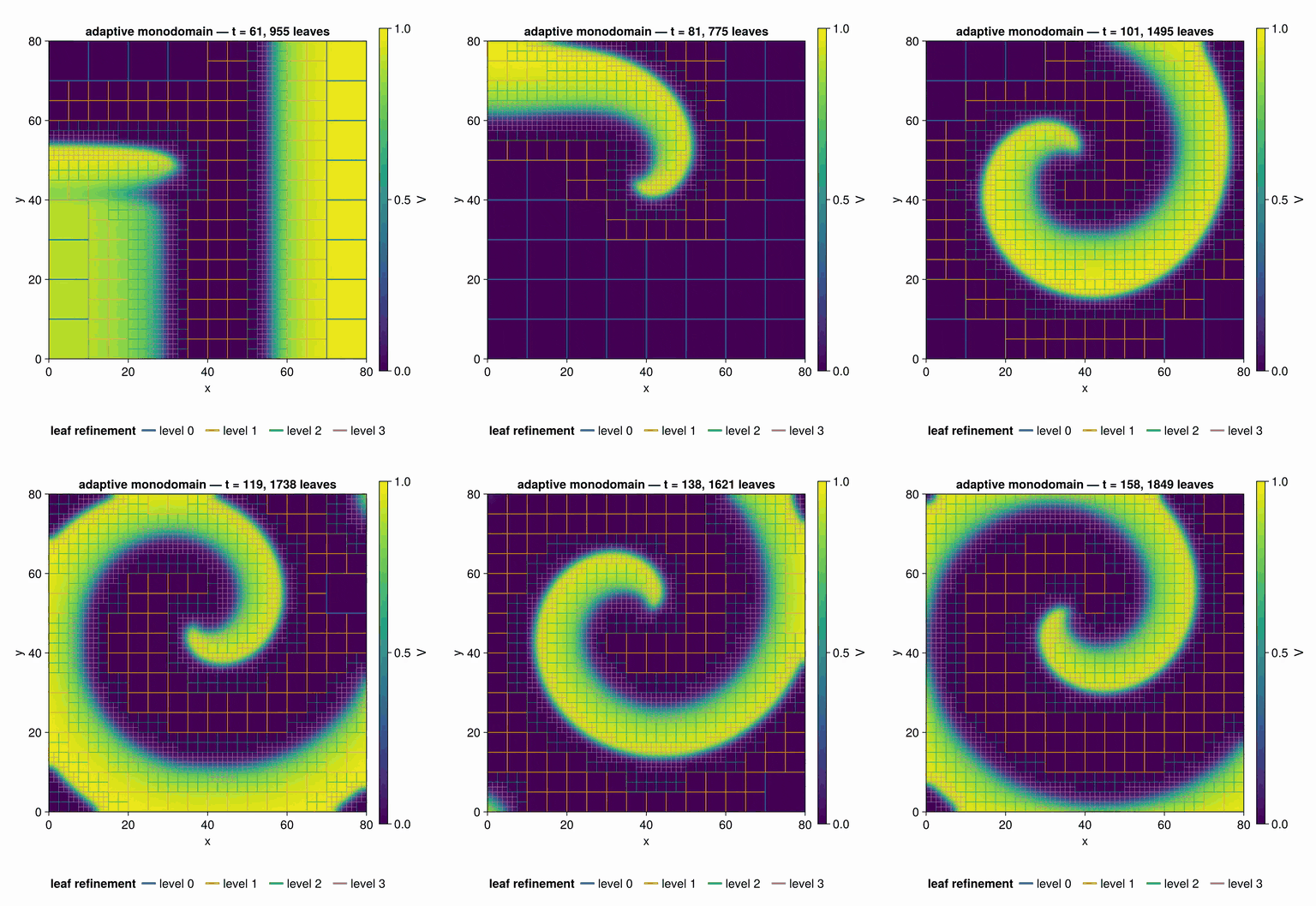
Animated cardiac electrophysiology simulation: a spiral wave rotating on an adaptively refined block mesh whose fine blocks track the wavefront. — Aliev–Panfilov monodomain cardiac electrophysiology on an adaptive `BlockForest`. `regrid!` refines on |∇V|, so resolution tracks the depolarization wavefront and coarsens behind it while an S1–S2 protocol breaks a planar wave into a reentrant spiral. Source: `examples/monodomain_amr.jl`.

Overview

MatrixFreeOperators.jl provides matrix-free linear (and some nonlinear) operators for solving PDEs on structured grids. Operators are lazy, composable symbols (laplacian, gradient, divergence, scaling, advection, …) combined with +, -, *, and scalar scaling. Leaves are written as array-level broadcasts, so the same operator runs on CPU and GPU arrays, differentiates automatically — Enzyme is the default backend, DifferentiationInterface the recommended frontend, and gradients extend to operator parameters such as material-coefficient fields (see Automatic Differentiation) — and feeds Krylov.jl directly through prepare + mul! with zero steady-state allocations. When one device is not enough, prepare_distributed partitions the grid across several GPUs without changing a line of operator code — see Distributed Multi-GPU Solves.

Quickstart

using MatrixFreeOperators, Krylov, LinearAlgebra

# -Δu + σu = f on (0,1)², homogeneous Dirichlet, manufactured solution
g = CartesianGrid(((0.0, 1.0), (0.0, 1.0)), (32, 32))
σ = set!(scalar_field(g), x -> 1 + x[1] * x[2])
K = scaling(σ) - laplacian(g)

f = set!(scalar_field(g), x -> (2π^2 + 1 + x[1] * x[2]) * sinpi(x[1]) * sinpi(x[2]))
P = prepare(K, scalar_field(g))
u, stats = cg(P, flatten(f))

maximum(abs, u .- flatten(set!(scalar_field(g), x -> sinpi(x[1]) * sinpi(x[2]))))

0.0007541253359055755